bayesml.sparselinearregression package

Module contents

This module provides the sparse linear regression model with the Laplace prior distribution (represented as a Gaussian scale mixture).

Stochastic Data Generative Model

The stochastic data generative model is as follows:

• \(d \in \mathbb{N}\): a dimension of explanatory variables

• \(\boldsymbol{x} \in \mathbb{R}^d\): an explanatory variable. If you consider an intercept term, it should be included as one of the elements of \(\boldsymbol{x}\).

• \(y \in \mathbb{R}\): an objective variable

• \(\boldsymbol{\theta} \in \mathbb{R}^d\): a regression coefficient vector

• \(\tau \in \mathbb{R}_{>0}\): a precision parameter

• \(\boldsymbol{v} = (v_1, \ldots, v_d)^\top \in \mathbb{R}_{>0}^d\): latent scale variables

\[\begin{split}p(y | \boldsymbol{x}, \boldsymbol{\theta}, \tau) &= \mathcal{N}(y | \boldsymbol{x}^{\top}\boldsymbol{\theta}, \tau^{-1}) \\ &= \sqrt{\frac{\tau}{2\pi}} \exp\left\{ -\frac{\tau}{2}(y-\boldsymbol{x}^{\top}\boldsymbol{\theta})^2 \right\}.\end{split}\]

\[\begin{split}\mathbb{E}[y | \boldsymbol{x}, \boldsymbol{\theta}, \tau] &= \boldsymbol{x}^{\top}\boldsymbol{\theta}, \\ \mathbb{V}[y | \boldsymbol{x}, \boldsymbol{\theta}, \tau] &= \tau^{-1}.\end{split}\]

Prior Distribution

The prior distribution is as follows:

• \(\boldsymbol{\lambda}_0 = (\lambda_{0,1}, \ldots, \lambda_{0,d})^\top \in \mathbb{R}_{>0}^d\): a hyperparameter vector (Laplace regularization strength for each dimension)

• \(\alpha_0 \in \mathbb{R}_{>0}\): a hyperparameter

• \(\beta_0 \in \mathbb{R}_{>0}\): a hyperparameter

• \(\Gamma(\cdot)\): the gamma function

\[\begin{split}p(\boldsymbol{\theta} | \tau, \boldsymbol{v}) &= \mathcal{N}(\boldsymbol{\theta} | \boldsymbol{0}, \tau^{-1} \mathrm{diag}(\boldsymbol{v})) \\ &= \left(\frac{\tau}{2\pi}\right)^{d/2} \left(\prod_{j=1}^d v_j\right)^{-1/2} \exp\left\{ -\frac{\tau}{2}\boldsymbol{\theta}^\top \mathrm{diag}(\boldsymbol{v})^{-1} \boldsymbol{\theta} \right\}, \\ p(\boldsymbol{v} | \boldsymbol{\lambda}_0) &= \prod_{j=1}^d \mathrm{Exp}\left(v_j \middle| \frac{\lambda_{0,j}^2}{2}\right) = \prod_{j=1}^d \frac{\lambda_{0,j}^2}{2}\exp\left(-\frac{\lambda_{0,j}^2}{2}v_j\right), \\ p(\tau | \alpha_0, \beta_0) &= \mathrm{Gam}(\tau | \alpha_0, \beta_0) = \frac{\beta_0^{\alpha_0}}{\Gamma(\alpha_0)}\tau^{\alpha_0-1}\exp(-\beta_0\tau).\end{split}\]

Marginalizing out each \(v_j\) yields the Laplace prior on \(\theta_j\):

\[\begin{split}p(\theta_j | \tau, \lambda_{0,j}) &= \int_0^\infty p(\theta_j | \tau, v_j) p(v_j | \lambda_{0,j})\, dv_j \\ &= \frac{\lambda_{0,j} \sqrt{\tau}}{2} \exp\left(-\lambda_{0,j} \sqrt{\tau}\, |\theta_j|\right).\end{split}\]

Posterior Distribution

The approximate posterior distribution in the \(t\)-th iteration of a variational Bayesian method is as follows:

• \(\boldsymbol{X} = (\boldsymbol{x}_1, \ldots, \boldsymbol{x}_n)^\top \in \mathbb{R}^{n \times d}\): given explanatory variables

• \(\boldsymbol{y} = (y_1, \ldots, y_n)^\top \in \mathbb{R}^n\): given objective variables

• \(\boldsymbol{\mu}_n^{(t)} \in \mathbb{R}^d\): a hyperparameter

• \(\boldsymbol{\Lambda}_n^{(t)} \in \mathbb{R}^{d \times d}\): a hyperparameter (a positive definite matrix)

• \(\alpha_n^{(t)} \in \mathbb{R}_{>0}\): a hyperparameter

• \(\beta_n^{(t)} \in \mathbb{R}_{>0}\): a hyperparameter

• \(a_{n,j}^{(t)} \in \mathbb{R}_{>0}\): a hyperparameter for \(q(v_j)\)

• \(b_{n,j}^{(t)} \in \mathbb{R}_{>0}\): a hyperparameter for \(q(v_j)\)

• \(K_{\nu}(\cdot)\): the modified Bessel function of the second kind

\[\begin{split}&q(\boldsymbol{\theta}, \tau, \boldsymbol{v}) \nonumber \\ &= \mathcal{N}\left( \boldsymbol{\theta} \middle| \boldsymbol{\mu}_n^{(t)}, (\tau \boldsymbol{\Lambda}_n^{(t)})^{-1} \right) \mathrm{Gam}(\tau | \alpha_n^{(t)}, \beta_n^{(t)}) \prod_{j=1}^d \mathrm{GIG}\left( v_j \middle| 1/2,\, a_{n,j}^{(t)},\, b_{n,j}^{(t)} \right) \\ &= \frac{|\tau \boldsymbol{\Lambda}_n^{(t)}|^{1/2}}{(2\pi)^{d/2}} \exp \left\{ -\frac{\tau}{2}(\boldsymbol{\theta} -\boldsymbol{\mu}_n^{(t)})^\top \boldsymbol{\Lambda}_n^{(t)} (\boldsymbol{\theta} - \boldsymbol{\mu}_n^{(t)}) \right\} \\ &\qquad \times \frac{(\beta_n^{(t)})^{\alpha_n^{(t)}}}{\Gamma(\alpha_n^{(t)})}\tau^{\alpha_n^{(t)}-1}\exp\{-\beta_n^{(t)}\tau\} \nonumber \\ &\qquad \times \prod_{j=1}^d \frac{(a_{n,j}^{(t)}/b_{n,j}^{(t)})^{1/4}}{2K_{1/2}\left(\sqrt{a_{n,j}^{(t)} b_{n,j}^{(t)}}\right)} v_j^{-1/2} \exp\left\{-\frac{1}{2}(a_{n,j}^{(t)} v_j + b_{n,j}^{(t)} v_j^{-1})\right\}\end{split}\]

where \(\mathrm{GIG}(x | p, a, b) = \frac{(a/b)^{p/2}}{2K_p(\sqrt{ab})} x^{p-1} \exp\left\{-\frac{1}{2}(ax + bx^{-1})\right\}\).

The updating rule of the hyperparameters is as follows.

\[\begin{split}\boldsymbol{\Lambda}_n^{(t+1)} &= \boldsymbol{X}^\top \boldsymbol{X} + \mathrm{diag}\left( \sqrt{\frac{a_{n,1}^{(t)}}{b_{n,1}^{(t)}}}, \ldots, \sqrt{\frac{a_{n,d}^{(t)}}{b_{n,d}^{(t)}}} \right), \\ \boldsymbol{\mu}_n^{(t+1)} &= (\boldsymbol{\Lambda}_n^{(t+1)})^{-1} \boldsymbol{X}^\top \boldsymbol{y}, \\ \alpha_n^{(t+1)} &= \alpha_0 + \frac{n}{2}, \\ \beta_n^{(t+1)} &= \beta_0 + \frac{1}{2} \left( \boldsymbol{y}^\top \boldsymbol{y} - (\boldsymbol{\mu}_n^{(t+1)})^\top \boldsymbol{\Lambda}_n^{(t+1)} \boldsymbol{\mu}_n^{(t+1)} \right), \\ a_{n,j}^{(t+1)} &= \lambda_{0,j}^2, \\ b_{n,j}^{(t+1)} &= \frac{\alpha_n^{(t+1)}}{\beta_n^{(t+1)}} (\mu_{n,j}^{(t+1)})^2 + \left((\boldsymbol{\Lambda}_n^{(t+1)})^{-1}\right)_{jj}.\end{split}\]

Accordingly,

\[\begin{split}\mathbb{E}[\boldsymbol{\theta} | \boldsymbol{X}, \boldsymbol{y}] &\approx \boldsymbol{\mu}_n, \\ \mathbb{E}[\tau | \boldsymbol{X}, \boldsymbol{y}] &\approx \frac{\alpha_n}{\beta_n}.\end{split}\]

Predictive Distribution

The approximate predictive distribution is as follows:

• \(\boldsymbol{x}_{n+1} \in \mathbb{R}^d\): a new explanatory variable

• \(y_{n+1} \in \mathbb{R}\): a new objective variable

• \(m_{\mathrm{p}} \in \mathbb{R}\): a parameter of the predictive distribution

• \(\lambda_{\mathrm{p}} \in \mathbb{R}_{>0}\): a parameter of the predictive distribution

• \(\nu_{\mathrm{p}} \in \mathbb{R}_{>0}\): a parameter of the predictive distribution

\[\begin{split}&p(y_{n+1} | \boldsymbol{X}, \boldsymbol{y}, \boldsymbol{x}_{n+1}) \nonumber \\ &\approx \mathrm{St}\left(y_{n+1} | m_{\mathrm{p}}, \lambda_{\mathrm{p}}, \nu_{\mathrm{p}}\right) \nonumber \\ &= \frac{\Gamma (\nu_\mathrm{p} / 2 + 1/2 )}{\Gamma (\nu_\mathrm{p} / 2)} \left( \frac{\lambda_\mathrm{p}}{\pi \nu_\mathrm{p}} \right)^{1/2} \left( 1 + \frac{\lambda_\mathrm{p} (y_{n+1} - m_\mathrm{p})^2}{\nu_\mathrm{p}} \right)^{-\nu_\mathrm{p}/2 - 1/2},\end{split}\]

\[\begin{split}\mathbb{E}[y_{n+1} | \boldsymbol{X}, \boldsymbol{y}, \boldsymbol{x}_{n+1}] &\approx m_{\mathrm{p}} \quad (\nu_{\mathrm{p}} > 1), \\ \mathbb{V}[y_{n+1} | \boldsymbol{X}, \boldsymbol{y}, \boldsymbol{x}_{n+1}] &\approx \frac{1}{\lambda_{\mathrm{p}}} \frac{\nu_{\mathrm{p}}}{\nu_{\mathrm{p}} - 2} \quad (\nu_{\mathrm{p}} > 2),\end{split}\]

where the parameters are obtained from the hyperparameters of the posterior distribution as follows:

\[\begin{split}m_{\mathrm{p}} &= \boldsymbol{x}_{n+1}^{\top} \boldsymbol{\mu}_n, \\ \lambda_{\mathrm{p}} &= \frac{\alpha_n}{\beta_n}\left(1 + \boldsymbol{x}_{n+1}^{\top} \boldsymbol{\Lambda}_n^{-1} \boldsymbol{x}_{n+1}\right)^{-1}, \\ \nu_{\mathrm{p}} &= 2\alpha_n.\end{split}\]

Star Us on GitHub

If you found this page helpful, please consider giving us a star on GitHub.

It really helps the project grow.

Open the repo and hit ☆ Star in the top right!

Classes

class bayesml.sparselinearregression.GenModel(c_degree, theta_vec=None, tau=1.0, h_lambdas=None, h_alpha=1.0, h_beta=1.0, seed=None)

ベースクラス: Generative

The stochastic data generative model and the prior distribution.

Parameters:

c_degreeint

A positive integer. The dimension of the explanatory variable. If you consider an intercept term, it should be included as one of the elements of the explanatory variable.

theta_vecnumpy ndarray, optional

A vector of real numbers, by default [0.0, ..., 0.0].

taufloat, optional

A positive real number, by default 1.0.

h_lambdasfloat or numpy.ndarray, optional

Positive real numbers, (Laplace regularization strength), by default [1.0, 1.0, ... , 1.0]. If a single real number is input, it will be broadcasted.

h_alphafloat, optional

A positive real number, by default 1.0.

h_betafloat, optional

A positive real number, by default 1.0.

seed{None, int}, optional

A seed to initialize numpy.random.default_rng(), by default None.

Methods

gen_params()	Generate parameters from the prior distribution.
gen_sample([sample_size, x, constant])	Generate a sample from the stochastic data generative model.
get_constants()	Get constants of GenModel.
get_h_params()	Get the hyperparameters of the prior distribution.
get_params()	Get the parameters of the stochastic data generative model.
load_h_params(filename)	Load the hyperparameters to h_params.
load_params(filename)	Load the parameters saved by save_params.
save_h_params(filename)	Save the hyperparameters using python pickle module.
save_params(filename)	Save the parameters using python pickle module.
save_sample(filename[, sample_size, x, constant])	Save the generated sample as NumPy .npz format.
set_h_params([h_lambdas, h_alpha, h_beta])	Set the hyperparameters of the prior distribution.
set_params([theta_vec, tau])	Set the parameters of the stochastic data generative model.
visualize_model([sample_size, constant])	Visualize the stochastic data generative model and generated samples.

get_constants()

Get constants of GenModel.

Returns:

constantsdict of {str: int}

• "c_degree" : the value of self.c_degree

set_h_params(h_lambdas=None, h_alpha=None, h_beta=None)

Set the hyperparameters of the prior distribution.

Parameters:

h_lambdasfloat or numpy.ndarray, optional

Positive real numbers, (Laplace regularization strength), by default None. If a single real number is input, it will be broadcasted.

h_alphafloat, optional

A positive real number, by default None.

h_betafloat, optional

A positive real number, by default None.

get_h_params()

Get the hyperparameters of the prior distribution.

Returns:

h_paramsdict of {str: float}

• "h_lambdas" : The value of self.h_lambdas

• "h_alpha" : The value of self.h_alpha

• "h_beta" : The value of self.h_beta

gen_params()

Generate parameters from the prior distribution.

The generated values are set at self.theta_vec, self.tau, and self.v_vec.

set_params(theta_vec=None, tau=None)

Set the parameters of the stochastic data generative model.

Parameters:

theta_vecnumpy ndarray, optional

A vector of real numbers, by default None.

taufloat, optional

A positive real number, by default None.

get_params()

Get the parameters of the stochastic data generative model.

Returns:

paramsdict of {str: float or numpy ndarray}

• "theta_vec" : The value of self.theta_vec

• "tau" : The value of self.tau

gen_sample(sample_size=None, x=None, constant=True)

Generate a sample from the stochastic data generative model.

If x is given, it will be used for explanatory variables as it is (independent of the other options: sample_size and constant).

If x is not given, it will be generated from i.i.d. standard normal distributions. The size of the generated sample is defined by sample_size. If constant is True, the last element of the generated explanatory variables will be overwritten by 1.0.

Parameters:

sample_sizeint, optional

A positive integer, by default None.

xnumpy ndarray, optional

A float array whose shape is (sample_size, c_degree), by default None.

constantbool, optional

A boolean value, by default True.

Returns:

xnumpy ndarray

A float array whose shape is (sample_size, c_degree).

ynumpy ndarray

A 1-dimensional float array whose size is sample_size.

save_sample(filename, sample_size=None, x=None, constant=True)

Save the generated sample as NumPy .npz format.

The generated sample is saved as a NpzFile with keywords "x" and "y".

Parameters:

filenamestr

The filename to which the sample is saved. .npz will be appended if it is not there.

sample_sizeint, optional

A positive integer, by default None.

xnumpy ndarray, optional

A float array whose shape is (sample_size, c_degree), by default None.

constantbool, optional

A boolean value, by default True.

参考

numpy.savez_compressed

visualize_model(sample_size=100, constant=True)

Visualize the stochastic data generative model and generated samples.

Parameters:

sample_sizeint, optional

A positive integer, by default 100.

constantbool, optional

A boolean value, by default True.

Examples

>>> import numpy as np
>>> from bayesml import sparselinearregression
>>> model = sparselinearregression.GenModel(
...     c_degree=2,
...     theta_vec=np.array([2.0, 1.0])
... )
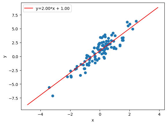
>>> model.visualize_model()

class bayesml.sparselinearregression.LearnModel(c_degree, h0_lambdas=None, h0_alpha=1.0, h0_beta=1.0, seed=None)

ベースクラス: Posterior, PredictiveMixin

The posterior distribution and the predictive distribution.

Inference is performed by variational Bayes. The variational posterior is

Parameters:

c_degreeint

A positive integer. The dimension of the explanatory variable.

h0_lambdasfloat, optional

Positive real numbers, (Laplace regularization strength), by default [1.0, 1.0, ... , 1.0]. If a single real number is input, it will be broadcasted.

h0_alphafloat, optional

A positive real number, by default 1.0.

h0_betafloat, optional

A positive real number, by default 1.0.

seed{None, int}, optional

A seed to initialize numpy.random.default_rng() used for VB random restarts, by default None.

Attributes:

hn_mu_vecnumpy ndarray

A vector of real numbers.

hn_lambda_matnumpy ndarray

A positive definite matrix.

hn_alphafloat

A positive real number.

hn_betafloat

A positive real number.

hn_asnumpy ndarray

A vector of positive real numbers (\(= \lambda_0^2\)).

hn_bsnumpy ndarray

A vector of positive real numbers.

p_msfloat

A real number.

p_lambdasfloat

A positive real number.

p_nusfloat

A positive real number.

vlfloat

The variational lower bound.

Methods

calc_pred_dist(x)	Calculate the parameters of the predictive distribution.
estimate_params([loss, dict_out])	Estimate the parameter of the stochastic data generative model under the given criterion.
fit(x, y[, max_itr, num_init, tolerance])	Fit the model to the data.
get_constants()	Get constants of LearnModel.
get_h0_params()	Get the initial values of the hyperparameters of the prior distribution.
get_hn_params()	Get the hyperparameters of the posterior distribution.
get_p_params()	Get the parameters of the predictive distribution.
load_h0_params(filename)	Load the hyperparameters to h0_params.
load_hn_params(filename)	Load the hyperparameters to hn_params.
make_prediction([loss])	Predict a new data point under the given criterion.
overwrite_h0_params()	Overwrite the initial values of the hyperparameters of the prior distribution by the learned values.
pred_and_update(x, y[, max_itr, num_init, ...])	Predict a new data point and update the posterior sequentially.
predict(x)	Predict the data.
reset_hn_params()	Reset the hyperparameters of the posterior distribution to initial values.
save_h0_params(filename)	Save the hyperparameters using python pickle module.
save_hn_params(filename)	Save the hyperparameters using python pickle module.
set_h0_params([h0_lambdas, h0_alpha, h0_beta])	Set initial values of the hyperparameters of the prior distribution.
set_hn_params([hn_mu_vec, hn_lambda_mat, ...])	Set updated values of the hyperparameters of the posterior distribution.
update_posterior(x, y[, max_itr, num_init, ...])	Update the hyperparameters of the posterior distribution using training data.
visualize_posterior()	Visualize the posterior distribution for the parameter.

get_constants()

Get constants of LearnModel.

Returns:

constantsdict of {str: int}

• "c_degree" : the value of self.c_degree

set_h0_params(h0_lambdas=None, h0_alpha=None, h0_beta=None)

Set initial values of the hyperparameters of the prior distribution.

Note that reset_hn_params() is called inside this method.

Parameters:

h0_lambdasfloat, optional

Positive real numbers, (Laplace regularization strength), by default None. If a single real number is input, it will be broadcasted.

h0_alphafloat, optional

A positive real number, by default None.

h0_betafloat, optional

A positive real number, by default None.

get_h0_params()

Get the initial values of the hyperparameters of the prior distribution.

Returns:

h0_paramsdict of {str: float}

• "h0_lambdas" : The value of self.h0_lambdas

• "h0_alpha" : The value of self.h0_alpha

• "h0_beta" : The value of self.h0_beta

reset_hn_params()

Reset the hyperparameters of the posterior distribution to initial values.

Usualy, hn_params are reset to the output of self.get_h0_params(), but the prior distribution and the posterior distribution have different form in this model, therefore, they are set to the solution of variational Bayesian updating formula with no data.

Note that calc_pred_dist is called with a zero vector inside this method.

overwrite_h0_params()

Overwrite the initial values of the hyperparameters of the prior distribution by the learned values.

Usualy, h0_params are overwritten to the output of self.get_hn_params(), but the prior distribution and the posterior distribution have different form in this model, therefore, h0_lambdas are set to minimize KL(GIG(1/2,`hn_as`,`hn_bs`)||Exp(0.5*`h0_lambdas`**2)).

Note that reset_hn_params() is called inside this method.

set_hn_params(hn_mu_vec=None, hn_lambda_mat=None, hn_alpha=None, hn_beta=None, hn_as=None, hn_bs=None)

Set updated values of the hyperparameters of the posterior distribution.

Note that calc_pred_dist is called with a zero vector inside this method.

Parameters:

hn_mu_vecnumpy ndarray, optional

A vector of real numbers, by default None.

hn_lambda_matnumpy ndarray, optional

A positive definite matrix, by default None.

hn_alphafloat, optional

A positive real number, by default None.

hn_betafloat, optional

A positive real number, by default None.

hn_asnumpy ndarray, optional

A vector of positive real numbers, by default None.

hn_bsnumpy ndarray, optional

A vector of positive real numbers, by default None.

get_hn_params()

Get the hyperparameters of the posterior distribution.

Returns:

hn_paramsdict of {str: float or numpy ndarray}

• "hn_mu_vec" : The value of self.hn_mu_vec

• "hn_lambda_mat" : The value of self.hn_lambda_mat

• "hn_alpha" : The value of self.hn_alpha

• "hn_beta" : The value of self.hn_beta

• "hn_as" : The value of self.hn_as

• "hn_bs" : The value of self.hn_bs

update_posterior(x, y, max_itr=100, num_init=10, tolerance=1.0e-8, init_type='Ridge', initial_bs=None, warm_start=False)

Update the hyperparameters of the posterior distribution using training data.

Parameters:

xnumpy ndarray

A float array whose shape is (sample_size, c_degree). If you want to use a constant term, it should be included in x.

ynumpy ndarray

A 1-dimensional float array whose size is sample_size.

max_itrint, optional

Maximum number of VB iterations per initialization, by default 100.

num_initint, optional

Number of random restarts, by default 10. If init_type is 'Ridge', 'OLS', or 'manual' or warm_start is True this argument is ignored.

tolerancefloat, optional

Convergence threshold on relative change of VL, by default 1.0e-8.

init_typestr, optional

Initialization method for the variational Bayesian method, by default 'Ridge'. This function supports the following values: * 'Ridge' : Initialize hn_mu_vec and hn_lambda_mat to the Ridge solution with h0_lambdas as the regularization strength. * 'OLS' : Initialize hn_mu_vec and hn_lambda_mat to the OLS solution. * 'exponential_rv' : Randomly initialize hn_bs from an exponential distribution with scale 1.0. * 'manual' : Manually set initial values of hn_bs. In this case, the argument initial_bs must be given.

initial_bsnumpy ndarray, optional

A vector of positive real numbers, by default None. If init_type is 'manual', this argument must be given.

warm_startbool, optional

If True, use the sufficient statistics of past samples and the current posterior as the starting point for the next update.

estimate_params(loss='squared', dict_out=False)

Estimate the parameter of the stochastic data generative model under the given criterion.

Note that the criterion is applied to estimating theta_vec and tau independently.

Parameters:

lossstr, optional

Loss function underlying the Bayes risk function, by default "squared". This function supports "squared", "0-1", "abs", and "KL".

dict_outbool, optional

If True, output will be a dict, by default False.

Returns:

estimatestuple of {numpy ndarray, float, None, or rv_frozen}

• theta_vec : the estimate for theta

• tau_hat : the estimate for tau

The estimated values under the given loss function. If it does not exist, None will be returned. If the loss is "KL", the approximate posterior distribution itself will be returned as rv_frozen objects of scipy.stats.

参考

scipy.stats.rv_continuous

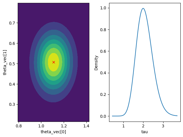
visualize_posterior()

Visualize the posterior distribution for the parameter.

Examples

>>> import numpy as np
>>> from bayesml import sparselinearregression
>>> gen_model = sparselinearregression.GenModel(
...     c_degree=2, theta_vec=np.array([1.0, 0.5]), tau=2.0, seed=0
... )
>>> x, y = gen_model.gen_sample(sample_size=50)
>>> learn_model = sparselinearregression.LearnModel(c_degree=2)
>>> learn_model.update_posterior(x, y)
>>> learn_model.visualize_posterior()

get_p_params()

Get the parameters of the predictive distribution.

Returns:

p_paramsdict of {str: float}

• "p_ms" : The value of self.p_ms

• "p_lambdas" : The value of self.p_lambdas

• "p_nus" : The value of self.p_nus

calc_pred_dist(x)

Calculate the parameters of the predictive distribution.

Parameters:

xnumpy ndarray

float array. The size along the last dimension must conincides with the c_degree. If you want to use a constant term, it should be included in x.

make_prediction(loss='squared')

Predict a new data point under the given criterion.

Parameters:

lossstr, optional

Loss function underlying the Bayes risk function, by default "squared". This function supports "squared", "0-1", "abs", and "KL".

Returns:

Predicted_values{numpy ndarray, rv_frozen}

The predicted values under the given loss function. The size of the predicted values is the same as the sample size of x when you called calc_pred_dist(x). If the loss function is "KL", the predictive distribution itself will be returned as rv_frozen object of scipy.stats. The rv_frozen object supports broadcasting.

参考

scipy.stats.rv_continuous

pred_and_update(x, y, max_itr=100, num_init=10, tolerance=1.0e-8, loss='squared')

Predict a new data point and update the posterior sequentially.

Note that update_posterior is called with warm_start=True inside this method.

Parameters:

xnumpy ndarray

A float array whose shape is (sample_size, c_degree). If you want to use a constant term, it should be included in x.

ynumpy ndarray

A 1-dimensional float array whose size is sample_size.

max_itrint, optional

Maximum number of VB iterations per initialization, by default 100.

num_initint, optional

Number of random restarts, by default 10.

tolerancefloat, optional

Convergence threshold on relative change of VL, by default 1.0e-8.

lossstr, optional

Loss function underlying the Bayes risk function, by default "squared".

Returns:

Predicted_values{numpy ndarray, rv_frozen}

The predicted values under the given loss function. The size of the predicted values is the same as the sample size of x when you called calc_pred_dist(x). If the loss function is "KL", the predictive distribution itself will be returned as rv_frozen object of scipy.stats.

参考

scipy.stats.rv_continuous

fit(x, y, max_itr=1000, num_init=10, tolerance=1.0E-8)

Fit the model to the data.

This function is a wrapper of the following functions:

>>> self.reset_hn_params()
>>> self.update_posterior(x,y,max_itr,tolerance)
>>> return self

Parameters:

xnumpy ndarray

float array. The size along the last dimension must conincides with the c_degree. If you want to use a constant term, it should be included in x.

ynumpy ndarray

float array.

max_itrint, optional

maximum number of iterations, by default 1000

num_initint, optional

number of initializations, by default 10

tolerancefloat, optional

convergence criterion of variational lower bound, by default 1.0E-8

Returns:

selfLearnModel

The fitted model.

predict(x)

Predict the data.

This function is a wrapper of the following functions:

>>> self.calc_pred_dist(x)
>>> return self.make_prediction(loss="squared")

Parameters:

xnumpy ndarray

float array. The size along the last dimension must conincides with the c_degree. If you want to use a constant term, it should be included in x.

Returns:

Predicted_valuesnumpy ndarray

The predicted values under the squared loss function. The size of the predicted values is the same as the sample size of x.