bayesml.linearregressionmixture package#
Module contents#
The mixture of linear regression model with the Gauss-Gamma prior distribution and the Dirichlet prior distribution.
The stochastic data generative model is as follows:
\(K \in \mathbb{N}\): number of latent classes
\(\boldsymbol{z} \in \{ 0, 1 \}^K\): a one-hot vector representing the latent class (latent variable)
\(\boldsymbol{\pi} \in [0, 1]^K\): a parameter for latent classes, (\(\sum_{k=1}^K \pi_k=1\))
\(D \in \mathbb{N}\): a dimension of data
\(y\in\mathbb{R}\): an objective variable
\(\boldsymbol{x} \in \mathbb{R}^D\): a data point
\(\boldsymbol{\theta}_k\in\mathbb{R}^{D}\): a parameter
\(\boldsymbol{\theta} = \{ \boldsymbol{\theta}_k \}_{k=1}^K\)
\(\tau_k \in \mathbb{R}_{>0}\) : a parameter
\(\boldsymbol{\tau} = \{ \tau_k \}_{k=1}^K\)
The prior distribution is as follows:
\(\boldsymbol{\mu}_0 \in \mathbb{R}^{D}\): a hyperparameter
\(\boldsymbol{\Lambda}_0 \in \mathbb{R}^{D\times D}\): a hyperparameter (a positive definite matrix)
\(\alpha_0 \in \mathbb{R}_{> 0}\): a hyperparameter
\(\beta_0\in \mathbb{R}_{>0}\): a hyperparameter
\(\boldsymbol{\gamma}_0 \in \mathbb{R}_{>0}^K\): a hyper parameter
\(\Gamma (\cdot)\): the gamma function
where \(C(\boldsymbol{\gamma}_0)\) are defined as follows:
The apporoximate posterior distribution in the \(t\)-th iteration of a variational Bayesian method is as follows:
\(\boldsymbol{X} = [\boldsymbol{x}_1, \boldsymbol{x}_2, \dots , \boldsymbol{x}_n]^\top \in \mathbb{R}^{n \times D}\): given explanatory variables
\(\boldsymbol{z}^n = (\boldsymbol{z}_1, \boldsymbol{z}_2, \dots , \boldsymbol{z}_n) \in \{ 0, 1 \}^{K \times n}\): latent classes of given data
\(\boldsymbol{r}_i^{(t)} = (r_{i,1}^{(t)}, r_{i,2}^{(t)}, \dots , r_{i,K}^{(t)}) \in [0,1]^K\): a parameter for \(i\)-th latent class (\(\sum_{k=1}^K r_{i,k}^{(t)} = 1\))
\(\boldsymbol{y} = [y_1, y_2, \dots , y_n]^\top \in \mathbb{R}^n\): given objective variables
\(\boldsymbol{\mu}_{n,k}^{(t)} \in \mathbb{R}^{D}\): a hyperparameter
\(\boldsymbol{\Lambda}_{n,k}^{(t)} \in \mathbb{R}^{D\times D}\): a hyperparameter (a positive definite matrix)
\(\alpha_{n,k}^{(t)} \in \mathbb{R}_{> 0}\): a hyperparameter
\(\beta_{n,k}^{(t)} \in \mathbb{R}_{>0}\): a hyperparameter
\(\boldsymbol{\gamma}_n^{(t)} \in \mathbb{R}_{>0}^K\): a hyper parameter
\(\psi (\cdot)\): the digamma function
where the updating rules of the hyperparameters are as follows:
The predictive distribution is as follows:
\(\boldsymbol{x}_{n+1}\in \mathbb{R}^D\): a new data point
\(y_{n+1}\in \mathbb{R}\): a new objective variable
\(m_{\mathrm{p},k}\in \mathbb{R}\): a parameter
\(\lambda_{\mathrm{p},k}\in \mathbb{R}_{>0}\): a parameter
\(\nu_{\mathrm{p},k}\in \mathbb{R}_{>0}\): a parameter
where the parameters are obtained from the hyperparameters of the posterior distribution as follows.
- class bayesml.linearregressionmixture.GenModel(c_num_classes, c_degree, *, pi_vec=None, theta_vecs=None, taus=None, h_gamma_vec=None, h_mu_vecs=None, h_lambda_mats=None, h_alphas=None, h_betas=None, seed=None)#
Bases:
GenerativeThe stochastic data generative model and the prior distribution
- Parameters:
- c_num_classesint
A positive integer
- c_degreeint
A positive integer
- pi_vecnumpy.ndarray, optional
A vector of real numbers in \([0, 1]\), by default [1/c_num_classes, 1/c_num_classes, … , 1/c_num_classes] Sum of its elements must be 1.0.
- theta_vecsnumpy.ndarray, optional
Vectors of real numbers, by default zero vectors.
- tausfloat or numpy.ndarray, optional
Positive real numbers, by default [1.0, 1.0, … , 1.0] If a single real number is input, it will be broadcasted.
- h_gamma_vecfloat or numpy.ndarray, optional
A vector of positive real numbers, by default [1/2, 1/2, … , 1/2] If a single real number is input, it will be broadcasted.
- h_mu_vecsnumpy.ndarray, optional
Vectors of real numbers, by default zero vectors
- h_lambda_matsnumpy.ndarray, optional
Positive definite symetric matrices, by default the identity matrices. If a single matrix is input, it will be broadcasted.
- h_alphasfloat or numpy.ndarray, optional
Positive real numbers, by default [1.0, 1.0, … , 1.0] If a single real number is input, it will be broadcasted.
- h_betasfloat or numpy.ndarray, optional
Positive real numbers, by default [1.0, 1.0, … , 1.0] If a single real number is input, it will be broadcasted.
- seed{None, int}, optional
A seed to initialize numpy.random.default_rng(), by default None
Methods
Generate the parameter from the prior distribution.
gen_sample([sample_size, x, constant])Generate a sample from the stochastic data generative model.
Get constants of GenModel.
Get the hyperparameters of the prior distribution.
Get the parameter of the sthocastic data generative model.
load_h_params(filename)Load the hyperparameters to h_params.
load_params(filename)Load the parameters saved by
save_params.save_h_params(filename)Save the hyperparameters using python
picklemodule.save_params(filename)Save the parameters using python
picklemodule.save_sample(filename[, sample_size, x, constant])Save the generated sample as NumPy
.npzformat.set_h_params([h_gamma_vec, h_mu_vecs, ...])Set the hyperparameters of the prior distribution.
set_params([pi_vec, theta_vecs, taus])Set the parameter of the sthocastic data generative model.
visualize_model([sample_size, constant])Visualize the stochastic data generative model and generated samples.
- get_constants()#
Get constants of GenModel.
- Returns:
- constantsdict of {str: int, numpy.ndarray}
"c_num_classes": the value ofself.c_num_classes"c_degree": the value ofself.c_degree
- set_params(pi_vec=None, theta_vecs=None, taus=None)#
Set the parameter of the sthocastic data generative model.
- Parameters:
- pi_vecnumpy.ndarray, optional
A vector of real numbers in \([0, 1]\), by default [1/c_num_classes, 1/c_num_classes, … , 1/c_num_classes] Sum of its elements must be 1.0.
- theta_vecsnumpy.ndarray, optional
Vectors of real numbers, by default zero vectors.
- tausfloat or numpy.ndarray, optional
Positive real numbers, by default [1.0, 1.0, … , 1.0] If a single real number is input, it will be broadcasted.
- set_h_params(h_gamma_vec=None, h_mu_vecs=None, h_lambda_mats=None, h_alphas=None, h_betas=None)#
Set the hyperparameters of the prior distribution.
- Parameters:
- h_gamma_vecfloat or numpy.ndarray, optional
A vector of positive real numbers, by default [1/2, 1/2, … , 1/2] If a single real number is input, it will be broadcasted.
- h_mu_vecsnumpy.ndarray, optional
Vectors of real numbers, by default zero vectors
- h_lambda_matsnumpy.ndarray, optional
Positive definite symetric matrices, by default the identity matrices. If a single matrix is input, it will be broadcasted.
- h_alphasfloat or numpy.ndarray, optional
Positive real numbers, by default [1.0, 1.0, … , 1.0] If a single real number is input, it will be broadcasted.
- h_betasfloat or numpy.ndarray, optional
Positive real numbers, by default [1.0, 1.0, … , 1.0] If a single real number is input, it will be broadcasted.
- get_params()#
Get the parameter of the sthocastic data generative model.
- Returns:
- params{str: numpy.ndarray}
"pi_vec": The value ofself.pi_vec"theta_vecs": The value ofself.theta_vecs"taus": The value ofself.taus
- get_h_params()#
Get the hyperparameters of the prior distribution.
- Returns:
- h_params{str:float, np.ndarray}
"h_gamma_vec": The value ofself.h_gamma_vec"h_mu_vecs": The value ofself.h_mu_vecs"h_lambda_mats": The value ofself.h_lambda_mats"h_alphas": The value ofself.h_alphas"h_betas": The value ofself.h_betas
- gen_params()#
Generate the parameter from the prior distribution.
The generated vaule is set at
self.pi_vec,self.theta_vecsandself.lambda_mats.
- gen_sample(sample_size=None, x=None, constant=True)#
Generate a sample from the stochastic data generative model.
If x is given, it will be used for explanatory variables as it is (independent of the other options: sample_size and constant).
If x is not given, it will be generated from i.i.d. standard normal distribution. The size of the generated sample is defined by sample_size. If constant is True, the last element of the generated explanatory variables will be overwritten by 1.0.
- Parameters:
- sample_sizeint, optional
A positive integer, by default
None.- xnumpy ndarray, optional
float array whose shape is
(sample_size,c_degree), by defaultNone.- constantbool, optional
A boolean value, by default
True.
- Returns:
- xnumpy ndarray
2-dimensional array whose shape is
(sample_size,c_degree)and its elements are real numbers.- znumpy ndarray
2-dimensional array whose shape is
(sample_size,c_num_classes)whose rows are one-hot vectors.- ynumpy ndarray
1 dimensional float array whose size is
sample_size.
- save_sample(filename, sample_size=None, x=None, constant=True)#
Save the generated sample as NumPy
.npzformat.If x is given, it will be used for explanatory variables as it is (independent of the other options: sample_size and constant).
If x is not given, it will be generated from i.i.d. standard normal distribution. The size of the generated sample is defined by sample_size. If constant is True, the last element of the generated explanatory variables will be overwritten by 1.0.
The generated sample is saved as a NpzFile with keyword: “x”, “z”, “y”.
- Parameters:
- filenamestr
The filename to which the sample is saved.
.npzwill be appended if it isn’t there.- sample_sizeint, optional
A positive integer, by default
None.- xnumpy ndarray, optional
float array whose shape is
(sample_size,c_degree), by defaultNone.- constantbool, optional
A boolean value, by default
True.
See also
- visualize_model(sample_size=100, constant=True)#
Visualize the stochastic data generative model and generated samples.
If x is given, it will be used for explanatory variables as it is (independent of the other options: sample_size and constant).
If x is not given, it will be generated from i.i.d. standard normal distribution. The size of the generated sample is defined by sample_size. If constant is True, the last element of the generated explanatory variables will be overwritten by 1.0.
- Parameters:
- sample_sizeint, optional
A positive integer, by default 100
- constantbool, optional
Examples
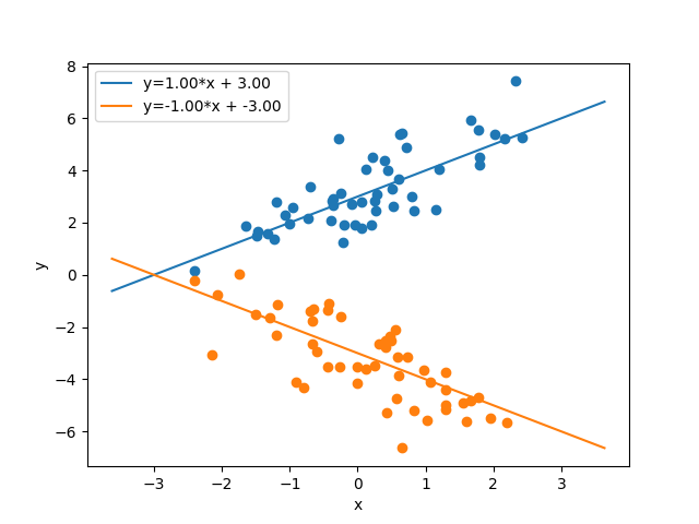
>>> from bayesml import linearregressionmixture
>>> import numpy as np
>>> model = linearregressionmixture.GenModel(
>>>     c_num_classes=2,
>>>     c_degree=2,
>>>     theta_vecs=np.array([[1,3],
>>>                          [-1,-3]]),
>>> )
>>> model.visualize_model()
pi_vec: [0.5 0.5] theta_vecs: [[ 1. 3.]
[-1. -3.]]
taus: [1. 1.]
- class bayesml.linearregressionmixture.LearnModel(c_num_classes, c_degree, *, h0_gamma_vec=None, h0_mu_vecs=None, h0_lambda_mats=None, h0_alphas=None, h0_betas=None, seed=None)#
Bases:
Posterior,PredictiveMixinThe posterior distribution and the predictive distribution.
- Parameters:
- c_num_classesint
a positive integer
- c_degreeint
a positive integer
- h0_gamma_vecfloat or numpy.ndarray, optional
A vector of positive real numbers, by default [1/2, 1/2, … , 1/2] If a single real number is input, it will be broadcasted.
- h0_mu_vecsnumpy.ndarray, optional
Vectors of real numbers, by default zero vectors
- h0_lambda_matsnumpy.ndarray, optional
Positive definite symetric matrices, by default the identity matrices. If a single matrix is input, it will be broadcasted.
- h0_alphasfloat or numpy.ndarray, optional
Positive real numbers, by default [1.0, 1.0, … , 1.0] If a single real number is input, it will be broadcasted.
- h0_betasfloat or numpy.ndarray, optional
Positive real numbers, by default [1.0, 1.0, … , 1.0] If a single real number is input, it will be broadcasted.
- seed{None, int}, optional
A seed to initialize numpy.random.default_rng(), by default None
- Attributes:
- hn_gamma_vecfloat or numpy.ndarray
A vector of positive real numbers. If a single real number is input, it will be broadcasted.
- hn_mu_vecsnumpy.ndarray
Vectors of real numbers.
- hn_lambda_matsnumpy.ndarray
Positive definite symetric matrices.
- hn_lambda_mats_invnumpy.ndarray
Positive definite symetric matrices.
- hn_alphasfloat or numpy.ndarray
Positive real numbers.
- hn_betasfloat or numpy.ndarray
Positive real numbers.
- r_vecsnumpy.ndarray
vectors of real numbers. The sum of its elenemts is 1.
- nsnumpy.ndarray
positive real numbers
- vlfloat
real number
- p_pi_vecsnumpy.ndarray
A vector of real numbers in \([0, 1]\). Sum of its elements must be 1.0.
- p_msnumpy.ndarray
Real numbers
- p_lambdasnumpy.ndarray
Positive real numbers
- p_nusnumpy.ndarray
Positive real numbers
Methods
Calculate the parameters of the predictive distribution.
estimate_latent_vars(x, y[, loss])Estimate latent variables corresponding to x under the given criterion.
estimate_latent_vars_and_update(x, y[, ...])Estimate latent variables and update the posterior sequentially.
estimate_params([loss])Estimate the parameter of the stochastic data generative model under the given criterion.
fit(x, y[, max_itr, num_init, tolerance, ...])Fit the model to the data.
Get constants of LearnModel.
Get the hyperparameters of the prior distribution.
Get the hyperparameters of the posterior distribution.
Get the parameters of the predictive distribution.
load_h0_params(filename)Load the hyperparameters to h0_params.
load_hn_params(filename)Load the hyperparameters to hn_params.
make_prediction([loss])Predict a new data point under the given criterion.
overwrite_h0_params()Overwrite the initial values of the hyperparameters of the posterior distribution by the learned values.
pred_and_update(x, y[, loss, max_itr, ...])Update the hyperparameters of the posterior distribution using traning data.
predict(x)Predict the data.
reset_hn_params()Reset the hyperparameters of the posterior distribution to their initial values.
save_h0_params(filename)Save the hyperparameters using python
picklemodule.save_hn_params(filename)Save the hyperparameters using python
picklemodule.set_h0_params([h0_gamma_vec, h0_mu_vecs, ...])Set the hyperparameters of the prior distribution.
set_hn_params([hn_gamma_vec, hn_mu_vecs, ...])Set the hyperparameter of the posterior distribution.
update_posterior(x, y[, max_itr, num_init, ...])Update the hyperparameters of the posterior distribution using traning data.
Visualize the posterior distribution for the parameter.
- get_constants()#
Get constants of LearnModel.
- Returns:
- constantsdict of {str: int, numpy.ndarray}
"c_num_classes": the value ofself.c_num_classes"c_degree": the value ofself.c_degree
- set_h0_params(h0_gamma_vec=None, h0_mu_vecs=None, h0_lambda_mats=None, h0_alphas=None, h0_betas=None)#
Set the hyperparameters of the prior distribution.
- Parameters:
- h0_gamma_vecfloat or numpy.ndarray, optional
A vector of positive real numbers, by default None. If a single real number is input, it will be broadcasted.
- h0_mu_vecsnumpy.ndarray, optional
Vectors of real numbers, by default None.
- h0_lambda_matsnumpy.ndarray, optional
Positive definite symetric matrices, by default the identity matrices. If a single matrix is input, it will be broadcasted.
- h0_alphasfloat or numpy.ndarray, optional
Positive real numbers, by default None. If a single real number is input, it will be broadcasted.
- h0_betasfloat or numpy.ndarray, optional
Positive real numbers, by default None. If a single real number is input, it will be broadcasted.
- get_h0_params()#
Get the hyperparameters of the prior distribution.
- Returns:
- h0_paramsdict of {str: numpy.ndarray}
"h0_gamma_vec": the value ofself.h0_gamma_vec"h0_mu_vecs": the value ofself.h0_mu_vecs"h0_lambda_mats": the value ofself.h0_lambda_mats"h0_alphas": the value ofself.h0_alphas"h0_betas": the value ofself.h0_betas
- set_hn_params(hn_gamma_vec=None, hn_mu_vecs=None, hn_lambda_mats=None, hn_alphas=None, hn_betas=None)#
Set the hyperparameter of the posterior distribution.
- Parameters:
- hn_gamma_vecfloat or numpy.ndarray, optional
A vector of positive real numbers, by default None. If a single real number is input, it will be broadcasted.
- hn_mu_vecsnumpy.ndarray, optional
Vectors of real numbers, by default None.
- hn_lambda_matsnumpy.ndarray, optional
Positive definite symetric matrices, by default the identity matrices. If a single matrix is input, it will be broadcasted.
- hn_alphasfloat or numpy.ndarray, optional
Positive real numbers, by default None. If a single real number is input, it will be broadcasted.
- hn_betasfloat or numpy.ndarray, optional
Positive real numbers, by default None. If a single real number is input, it will be broadcasted.
- get_hn_params()#
Get the hyperparameters of the posterior distribution.
- Returns:
- hn_paramsdict of {str: numpy.ndarray}
"hn_gamma_vec": the value ofself.hn_gamma_vec"hn_mu_vecs": the value ofself.hn_mu_vecs"hn_lambda_mats": the value ofself.hn_lambda_mats"hn_alphas": the value ofself.hn_alphas"hn_betas": the value ofself.hn_betas
- update_posterior(x, y, max_itr=100, num_init=10, tolerance=1e-08, init_type='random_responsibility')#
Update the hyperparameters of the posterior distribution using traning data.
- Parameters:
- xnumpy ndarray
float array. The size along the last dimension must conincides with the c_degree. If you want to use a constant term, it should be included in x.
- ynumpy ndarray
float array.
- max_itrint, optional
maximum number of iterations, by default 100
- num_initint, optional
number of initializations, by default 10
- tolerancefloat, optional
convergence criterion of variational lower bound, by default 1.0E-8
- init_typestr, optional
'random_responsibility': randomly assign responsibility tor_vecs'subsampling': for each latent class, extract a subsample whose size isint(np.sqrt(x.shape[0])). and use it to update q(theta_k,tau_k).
Type of initialization, by default
'random_responsibility'
- estimate_params(loss='squared')#
Estimate the parameter of the stochastic data generative model under the given criterion.
Note that the criterion is applied to estimating
pi_vec,theta_vecsandtausindependently. Therefore, a tuple of the dirichlet distribution, the student’s t-distributions and the wishart distributions will be returned when loss=”KL”- Parameters:
- lossstr, optional
Loss function underlying the Bayes risk function, by default “squared”. This function supports “squared”, “0-1”, and “KL”.
- Returns:
- Estimatesa tuple of {numpy ndarray, float, None, or rv_frozen}
pi_vec_hat: the estimate for pi_vectheta_vecs_hat: the estimate for theta_vecstaus_hat: the estimate for taus
The estimated values under the given loss function. If it is not exist, np.nan will be returned. If the loss function is “KL”, the posterior distribution itself will be returned as rv_frozen object of scipy.stats.
- visualize_posterior()#
Visualize the posterior distribution for the parameter.
Examples
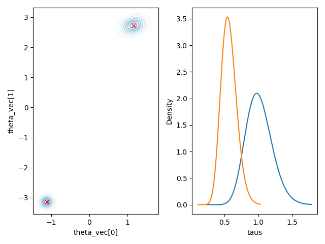
>>> import numpy as np
>>> from bayesml import linearregressionmixture
>>> gen_model = linearregressionmixture.GenModel(
>>>     c_num_classes=2,
>>>     c_degree=2,
>>>     theta_vecs=np.array([[1,3],[-1,-3]]),
>>>     taus=np.array([0.5,1.0]),
>>>     )
>>> x,z,y = gen_model.gen_sample(100)
>>> learn_model = linearregressionmixture.LearnModel(
>>>     c_num_classes=2,
>>>     c_degree=2,
>>>     )
>>> learn_model.update_posterior(x,y)
>>> learn_model.visualize_posterior()
hn_gamma_vec:
[53.46589867 47.53410133]
E[pi_vec]:
[0.52936533 0.47063467]
hn_mu_vecs:
[[-1.12057057 -3.14175971]
[ 1.15046197  2.72935847]]
hn_lambda_mats:
[[[ 73.28683786  -1.18874056]
[ -1.18874056  53.96589867]]
[[ 39.13313893 -10.37075427] [-10.37075427 48.03410133]]] hn_alphas: [27.48294934 24.51705066] hn_betas: [27.13542998 43.09024752] E[taus]: [1.01280685 0.56896983]
- get_p_params()#
Get the parameters of the predictive distribution.
- Returns:
- p_paramsdict of {str: numpy.ndarray}
"p_pi_vecs": the value ofself.p_pi_vecs"p_ms": the value ofself.p_ms"p_lambdas": the value ofself.p_lambdas"p_nus": the value ofself.p_nus
- calc_pred_dist(x)#
Calculate the parameters of the predictive distribution.
- Parameters:
- xnumpy ndarray
float array. The size along the last dimension must conincides with the c_degree. If you want to use a constant term, it should be included in x.
- make_prediction(loss='squared')#
Predict a new data point under the given criterion.
- Parameters:
- lossstr, optional
Loss function underlying the Bayes risk function, by default “squared”. This function supports “squared” and “0-1”.
- Returns:
- predicted_valuenumpy.ndarray
The predicted value under the given loss function. The size of the predicted values is the same as the sample size of x when you called calc_pred_dist(x).
- pred_and_update(x, y, loss='squared', max_itr=100, num_init=10, tolerance=1e-08, init_type='random_responsibility')#
Update the hyperparameters of the posterior distribution using traning data.
h0_params will be overwritten by current hn_params before updating hn_params by x
- Parameters:
- xnumpy ndarray
float array. The size along the last dimension must conincides with the c_degree. If you want to use a constant term, it should be included in x.
- ynumpy ndarray
float array.
- lossstr, optional
Loss function underlying the Bayes risk function, by default “squared”. This function supports “squared” and “0-1”.
- max_itrint, optional
maximum number of iterations, by default 100
- num_initint, optional
number of initializations, by default 10
- tolerancefloat, optional
convergence criterion of variational lower bound, by default 1.0E-8
- init_typestr, optional
'random_responsibility': randomly assign responsibility tor_vecs'subsampling': for each latent class, extract a subsample whose size isint(np.sqrt(x.shape[0])). and use it to update q(theta_k,tau_k).
Type of initialization, by default
'random_responsibility'
- Returns:
- predicted_valuenumpy.ndarray
The predicted value under the given loss function. The size of the predicted values is the same as the sample size of x when you called calc_pred_dist(x).
- fit(x, y, max_itr=1000, num_init=10, tolerance=1e-08, init_type='random_responsibility')#
Fit the model to the data.
This function is a wrapper of the following functions:
>>> self.reset_hn_params()
>>> self.update_posterior(x,y,max_itr,tolerance,init_type)
>>> return self
- Parameters:
- xnumpy ndarray
float array. The size along the last dimension must conincides with the c_degree. If you want to use a constant term, it should be included in x.
- ynumpy ndarray
float array.
- max_itrint, optional
maximum number of iterations, by default 1000
- num_initint, optional
number of initializations, by default 10
- tolerancefloat, optional
convergence criterion of variational lower bound, by default 1.0E-8
- init_typestr, optional
'random_responsibility': randomly assign responsibility tor_vecs'subsampling': for each latent class, extract a subsample whose size isint(np.sqrt(x.shape[0])). and use it to update q(theta_k,tau_k).
Type of initialization, by default
'random_responsibility'
- Returns:
- selfLearnModel
The fitted model.
- predict(x)#
Predict the data.
This function is a wrapper of the following functions:
>>> self.calc_pred_dist(x)
>>> return self.make_prediction(loss="squared")
- Parameters:
- xnumpy ndarray
float array. The size along the last dimension must conincides with the c_degree. If you want to use a constant term, it should be included in x.
- Returns:
- Predicted_valuesnumpy ndarray
The predicted values under the squared loss function. The size of the predicted values is the same as the sample size of x.
- estimate_latent_vars(x, y, loss='0-1')#
Estimate latent variables corresponding to x under the given criterion.
Note that the criterion is independently applied to each data point.
- Parameters:
- xnumpy ndarray
float array. The size along the last dimension must conincides with the c_degree. If you want to use a constant term, it should be included in x.
- ynumpy ndarray
float array.
- lossstr, optional
Loss function underlying the Bayes risk function, by default “0-1”. This function supports “squared”, “0-1”, and “KL”.
- Returns:
- estimatesnumpy.ndarray
The estimated values under the given loss function. If the loss function is “KL”, the posterior distribution will be returned as a numpy.ndarray whose elements consist of occurence probabilities.
- estimate_latent_vars_and_update(x, y, loss='0-1', max_itr=100, num_init=10, tolerance=1e-08, init_type='random_responsibility')#
Estimate latent variables and update the posterior sequentially.
h0_params will be overwritten by current hn_params before updating hn_params by x
- Parameters:
- xnumpy ndarray
float array. The size along the last dimension must conincides with the c_degree. If you want to use a constant term, it should be included in x.
- ynumpy ndarray
float array.
- lossstr, optional
Loss function underlying the Bayes risk function, by default “0-1”. This function supports “squared” and “0-1”.
- max_itrint, optional
maximum number of iterations, by default 100
- num_initint, optional
number of initializations, by default 10
- tolerancefloat, optional
convergence croterion of variational lower bound, by default 1.0E-8
- init_typestr, optional
'subsampling': for each latent class, extract a subsample whose size isint(np.sqrt(x.shape[0])). and use its mean and covariance matrix as an initial values ofhn_m_vecsandhn_lambda_mats.'random_responsibility': randomly assign responsibility tor_vecs
Type of initialization, by default
'subsampling'
- Returns:
- estimatesnumpy.ndarray
The estimated values under the given loss function. If the loss function is “KL”, the posterior distribution will be returned as a numpy.ndarray whose elements consist of occurence probabilities.