bayesml.metatree package

bayesml.metatree package#

Module contents#

Stochastic Data Generative Model#

$\boldsymbol{x}=[x_1, \ldots, x_p, x_{p+1}, \ldots , x_{p+q}]$ : an explanatory variable. The first $p$ variables are continuous. The other $q$ variables are categorical.
$\mathcal{Y}$ : a space of an objective variable
$y \in \mathcal{Y}$ : an objective variable
$D_\mathrm{max} \in \mathbb{N}$ : the maximum depth of trees
$T_\mathrm{max}$ : the perfect tree where all the inner nodes have the same number of child nodes and all the leaf nodes have the same depth of $D_\mathrm{max}$
$\mathcal{S}_\mathrm{max}$ : the set of all the nodes of $T_\mathrm{max}$
$s \in \mathcal{S}_\mathrm{max}$ : a node of a tree
$\mathcal{I}_\mathrm{max} \subset \mathcal{S}_\mathrm{max}$ : the set of all the inner nodes of $T_\mathrm{max}$
$\mathcal{L}_\mathrm{max} \subset \mathcal{S}_\mathrm{max}$ : the set of all the leaf nodes of $T_\mathrm{max}$
$\mathcal{T}$ : the set of all the pruned subtrees of $T_\mathrm{max}$
$T \in \mathcal{T}$ : a pruned subtree of $T_\mathrm{max}$
$\mathcal{I}_T$ : the set of all the inner nodes of $T$
$\mathcal{L}_T$ : the set of all the leaf nodes of $T$
$\boldsymbol{k}=(k_s)_{s \in \mathcal{I}_\mathrm{max}}$ : indices of the features assigned to inner nodes, i.e., $k_s \in \{1, 2,\ldots,p+q\}$. If $k_s \leq p$, the node $s$ has a threshold.
$\mathcal{K}=\{ 1, 2, \ldots , p+q \}^{|\mathcal{I}_\mathrm{max}|}$ : the set of all $\boldsymbol{k}$
$\boldsymbol{\theta}=(\theta_s)_{s \in \mathcal{S}}$ : parameters assigned to the nodes
$s_{\boldsymbol{k},T}(\boldsymbol{x}) \in \mathcal{L}_T$ : a leaf node which $\boldsymbol{x}$ reaches under $T$ and $\boldsymbol{k}$

\[p(y | \boldsymbol{x}, \boldsymbol{\theta}, T, \boldsymbol{k})=p(y | \theta_{s_{\boldsymbol{k},T}(\boldsymbol{x})})\]

Prior Distribution#

$g_s \in [0,1]$ : a hyperparameter assigned to each node $s \in \mathcal{S}_\mathrm{max}$. For any leaf node $s$ of $T_\mathrm{max}$, we assume $g_s=0$.

\[\begin{split}p(\boldsymbol{k}) &= \frac{1}{|\mathcal{K}|} = \left( \frac{1}{p+q} \right)^{|\mathcal{I}_\mathrm{max}|}, \\ p(T) &= \prod_{s \in \mathcal{I}_T} g_s \prod_{s' \in \mathcal{L}_T} (1-g_{s'}).\end{split}\]

The prior distribution of the parameter $\theta_s$ is assumed to be a conjugate prior distribution for $p(y | \theta_s)$ and independent for each node.

Posterior Distribution#

The posterior distribution is approximated as follows:

$n \in \mathbb{N}$ : a sample size
$\boldsymbol{x}^n = \{ \boldsymbol{x}_1, \boldsymbol{x}_2, \ldots, \boldsymbol{x}_n \}$
$\boldsymbol{x}_{s, \boldsymbol{k}}$ : the explanatory variables of the data points that pass through $s$ under $\boldsymbol{k}$.
$y^n = \{ y_1, y_2, \ldots, y_n \}$
$y_{s, \boldsymbol{k}}$ : the objective variables of the data points that pass through $s$ under $\boldsymbol{k}$.

First, the posterior distribution $p(\boldsymbol{k}, T, \boldsymbol{\theta} | \boldsymbol{x}^n, y^n)$ can be decomposed as follows:

\[p(\boldsymbol{k}, T, \boldsymbol{\theta} | \boldsymbol{x}^n, y^n) = p(\boldsymbol{k} | \boldsymbol{x}^n, y^n) p(T | \boldsymbol{x}^n, y^n, \boldsymbol{k}) p(\boldsymbol{\theta} | \boldsymbol{x}^n, y^n, \boldsymbol{k}, T).\]

For $\boldsymbol{\theta}$, we can exactly calculate the posterior distribution $p(\boldsymbol{\theta} | \boldsymbol{x}^n, y^n, \boldsymbol{k}, T)$ because we assumed the conjugate prior distribution.

Also for $T$, we can exactly calculate the posterior distribution $p(T | \boldsymbol{x}^n, y^n, \boldsymbol{k})$ by using the concept called a meta-tree. The meta-tree is not a tree but a set of trees where all the trees have the same feature assignment $\boldsymbol{k}$ to their inner nodes. The posterior distribution of the trees over the meta-tree defined by $\boldsymbol{k}$ is as follows:

\[p(T | \boldsymbol{x}^n, y^n, \boldsymbol{k}) = \prod_{s \in \mathcal{I}_T} g_{s|\boldsymbol{x}^n, y^n, \boldsymbol{k}} \prod_{s' \in \mathcal{L}_T} (1-g_{s'|\boldsymbol{x}^n, y^n, \boldsymbol{k}}),\]

where $g_{s|\boldsymbol{x}^n, y^n, \boldsymbol{k}} \in [0,1]$ can be calculated from $\boldsymbol{x}^n$, $y^n$, and $\boldsymbol{k}$ as follows:

\[\begin{split}g_{s|\boldsymbol{x}^n, y^n, \boldsymbol{k}} = \begin{cases} \frac{g_s \prod_{s' \in \mathrm{Ch}(s)}q(y_{s', \boldsymbol{k}}|\boldsymbol{x}_{s', \boldsymbol{k}}, s', \boldsymbol{k})}{q(y_{s, \boldsymbol{k}}|\boldsymbol{x}_{s, \boldsymbol{k}}, s, \boldsymbol{k})}, & s \in \mathcal{I}_\mathrm{max},\\ g_s, & \mathrm{otherwise}, \end{cases}\end{split}\]

where $\mathrm{Ch}(s)$ denotes the set of child nodes of $s$ on $T_\mathrm{max}$ and $q(y_{s, \boldsymbol{k}}|\boldsymbol{x}_{s, \boldsymbol{k}}, s, \boldsymbol{k})$ is defined for any $s \in \mathcal{S}_\mathrm{max}$ as follows.

\[\begin{split}&q(y_{s, \boldsymbol{k}}|\boldsymbol{x}_{s, \boldsymbol{k}}, s, \boldsymbol{k}) = \begin{cases} (1-g_s) f(y_{s, \boldsymbol{k}} | \boldsymbol{x}_{s, \boldsymbol{k}}, s, \boldsymbol{k}) \\ \qquad {}+ g_s \prod_{s' \in \mathrm{Ch}(s)} q(y_{s', \boldsymbol{k}} | \boldsymbol{x}_{s', \boldsymbol{k}}, s', \boldsymbol{k}), & s \in \mathcal{I}_\mathrm{max},\\ f(y_{s, \boldsymbol{k}} | \boldsymbol{x}_{s, \boldsymbol{k}}, s, \boldsymbol{k}), & \mathrm{otherwise}. \end{cases}\end{split}\]

Here, $f(y_{s, \boldsymbol{k}} | \boldsymbol{x}_{s, \boldsymbol{k}}, s, \boldsymbol{k})$ is defined as follows:

\[f(y_{s, \boldsymbol{k}} | \boldsymbol{x}_{s, \boldsymbol{k}}, s, \boldsymbol{k}) = \int p(y_{s, \boldsymbol{k}} | \boldsymbol{x}_{s, \boldsymbol{k}}, \theta_s) p(\theta_s) \mathrm{d}\theta_s.\]

For $\boldsymbol{k}$, there are two algirithms to approximate the posterior distribution $p(\boldsymbol{k} | \boldsymbol{x}^n, y^n)$: the meta-tree random forest (MTRF) and the meta-tree Markov chain Monte Carlo (MTMCMC) method.

Approximation by MTRF#

In MTRF, we first construct a set of feature assignment vectors $\mathcal{K}' = \{\boldsymbol{k}_1, \boldsymbol{k}_2, \ldots, \boldsymbol{k}_B\}$ by using the usual (non-Bayesian) random forest algorithm. Next, for $\boldsymbol{k} \in \mathcal{K}$, we approximate the posterior distribution $p(\boldsymbol{k} | \boldsymbol{x}^n, y^n)$ as follows:

\[\begin{split}p(\boldsymbol{k} | \boldsymbol{x}^n, y^n) \approx \tilde{p}(\boldsymbol{k} | \boldsymbol{x}^n, y^n) \propto \begin{cases} q(y_{s_\lambda, \boldsymbol{k}}|\boldsymbol{x}_{s_\lambda, \boldsymbol{k}}, s_\lambda, \boldsymbol{k}), & \boldsymbol{k} \in \mathcal{K}',\\ 0, & \mathrm{otherwise}. \end{cases}\end{split}\]

where $s_{\lambda}$ is the root node of $T_\mathrm{max}$.

The predictive distribution is approximated as follows:

\[p(y_{n+1}| \boldsymbol{x}_{n+1}, \boldsymbol{x}^n, y^n) = \sum_{\boldsymbol{k} \in \mathcal{K}'} \tilde{p}(\boldsymbol{k} | \boldsymbol{x}^n, y^n) q(y_{n+1}|\boldsymbol{x}_{n+1},\boldsymbol{x}^n, y^n, s_\lambda, \boldsymbol{k}),\]

where $q(y_{n+1}|\boldsymbol{x}_{n+1},\boldsymbol{x}^n, y^n, s_\lambda, \boldsymbol{k})$ is calculated in a similar manner to $q(y_{s_\lambda, \boldsymbol{k}}|\boldsymbol{x}_{s_\lambda, \boldsymbol{k}}, s_\lambda, \boldsymbol{k})$.

The expectation of the predictive distribution is approximated as follows.

\[\mathbb{E}_{p(y_{n+1}| \boldsymbol{x}_{n+1}, \boldsymbol{x}^n, y^n)} [Y_{n+1}| \boldsymbol{x}_{n+1}, \boldsymbol{x}^n, y^n] = \sum_{\boldsymbol{k} \in \mathcal{K}'} \tilde{p}(\boldsymbol{k} | \boldsymbol{x}^n, y^n) \mathbb{E}_{q(y_{n+1}|\boldsymbol{x}_{n+1},\boldsymbol{x}^n, y^n, s_\lambda, \boldsymbol{k})} [Y_{n+1}| \boldsymbol{x}_{n+1}, \boldsymbol{x}^n, y^n, \boldsymbol{k}],\]

where the expectation for $q$ is recursively given as follows.

\[\begin{split}&\mathbb{E}_{q(y_{n+1}|\boldsymbol{x}_{n+1},\boldsymbol{x}^n, y^n, s, \boldsymbol{k})} [Y_{n+1} | \boldsymbol{x}_{n+1}, \boldsymbol{x}^n, y^n, \boldsymbol{k}] \\ &= \begin{cases} (1-g_{s|\boldsymbol{x}^n, y^n, \boldsymbol{k}}) \mathbb{E}_{f(y_{n+1}|\boldsymbol{x}_{n+1},\boldsymbol{x}^n, y^n, s, \boldsymbol{k})} [Y_{n+1} | \boldsymbol{x}_{n+1}, \boldsymbol{x}^n, y^n, \boldsymbol{k}] \\ \qquad + g_{s|\boldsymbol{x}^n, y^n, \boldsymbol{k}} \mathbb{E}_{q(y_{n+1}|\boldsymbol{x}_{n+1},\boldsymbol{x}^n, y^n, s_\mathrm{child}, \boldsymbol{k})} [Y_{n+1} | \boldsymbol{x}_{n+1}, \boldsymbol{x}^n, y^n, \boldsymbol{k}] ,& s \in \mathcal{I}_\mathrm{max},\\ \mathbb{E}_{f(y_{n+1}|\boldsymbol{x}_{n+1},\boldsymbol{x}^n, y^n, s, \boldsymbol{k})} [Y_{n+1} | \boldsymbol{x}_{n+1}, \boldsymbol{x}^n, y^n, \boldsymbol{k}],& (\mathrm{otherwise}). \end{cases}\end{split}\]

Here, $f(y_{n+1}|\boldsymbol{x}_{n+1},\boldsymbol{x}^n, y^n, s, \boldsymbol{k})$ is calculated in a similar manner to $f(y_{s, \boldsymbol{k}} | \boldsymbol{x}_{s, \boldsymbol{k}}, s, \boldsymbol{k})$ and $s_\mathrm{child}$ is the child node of $s$ on the path from the root node to the leaf node $s_{\boldsymbol{k},T_\mathrm{max}}(\boldsymbol{x}_{n+1})$.

Approximation by MTMCMC#

In MTMCMC method, we generate a sample $\boldsymbol{k}$ from the posterior distribution $p(\boldsymbol{k} | \boldsymbol{x}^n, y^n)$ by a MCMC method, and the posterior distribution is approximated by the empirical distribution of this sample. Let $\{\boldsymbol{k}^{(t)}\}_{t=1}^{t_\mathrm{end}}$ be the obtained sample.

The predictive distribution is approximated as follows:

\[p(y_{n+1}| \boldsymbol{x}_{n+1}, \boldsymbol{x}^n, y^n) = \frac{1}{t_\mathrm{end}} \sum_{t=1}^{t_\mathrm{end}} q(y_{n+1}|\boldsymbol{x}_{n+1},\boldsymbol{x}^n, y^n, s_\lambda, \boldsymbol{k}^{(t)}).\]

The expectation of the predictive distribution is approximated as follows:

\[\mathbb{E}_{p(y_{n+1}| \boldsymbol{x}_{n+1}, \boldsymbol{x}^n, y^n)} [Y_{n+1}| \boldsymbol{x}_{n+1}, \boldsymbol{x}^n, y^n] = \frac{1}{t_\mathrm{end}} \sum_{t=1}^{t_\mathrm{end}} \mathbb{E}_{q(y_{n+1}|\boldsymbol{x}_{n+1},\boldsymbol{x}^n, y^n, s_\lambda, \boldsymbol{k}^{(t)})} [Y_{n+1}| \boldsymbol{x}_{n+1}, \boldsymbol{x}^n, y^n, \boldsymbol{k}^{(t)}].\]

References#

Dobashi, N.; Saito, S.; Nakahara, Y.; Matsushima, T. Meta-Tree Random Forest: Probabilistic Data-Generative Model and Bayes Optimal Prediction. Entropy 2021, 23, 768. https://doi.org/10.3390/e23060768
Nakahara, Y.; Saito, S.; Kamatsuka, A.; Matsushima, T. Probability Distribution on Full Rooted Trees. Entropy 2022, 24, 328. https://doi.org/10.3390/e24030328
Nakahara, Y.; Saito, S.; Ichijo, N.; Kazama, K.; Matsushima, T. Bayesian Decision Theory on Decision Trees: Uncertainty Evaluation and Interpretability. Proceedings of The 28th International Conference on Artificial Intelligence and Statistics, in Proceedings of Machine Learning Research 2025, 258:1045-1053 Available from https://proceedings.mlr.press/v258/nakahara25a.html.

class bayesml.metatree.GenModel(c_dim_continuous, c_dim_categorical, c_max_depth=2, c_num_children_vec=2, c_num_assignment_vec=None, c_ranges=None, SubModel=<module 'bayesml.bernoulli'>, sub_constants={}, root=None, h_k_weight_vec=None, h_g=0.5, sub_h_params={}, h_metatree_list=[], h_metatree_prob_vec=None, seed=None)#

Bases: Generative

The stochastice data generative model and the prior distribution

Parameters:

c_dim_continuousint: A non-negative integer
c_dim_categoricalint: A non-negative integer
c_num_children_vecnumpy.ndarray, optional: A vector of positive integers whose length is c_dim_continuous+c_dim_categorical, by default [2,2,…,2]. The first c_dim_continuous elements represent the numbers of children of continuous features at inner nodes. The other c_dim_categorial elements represent those of categorical features. If a single integer is input, it will be broadcasted.
c_max_depthint, optional: A positive integer, by default 2
c_num_assignment_vecnumpy.ndarray, optional: A vector of positive integers whose length is c_dim_continuous+c_dim_categorical. The first c_dim_continuous elements represent the maximum assignment numbers of continuous features on a path. The other c_dim_categorial elements represent those of categorical features. If it has a negative element (e.g., -1), the corresponding feature will be assigned any number of times. By default [-1,…,-1].
c_rangesnumpy.ndarray, optional: A numpy.ndarray whose size is (c_dim_continuous,2). A threshold for the k-th continuous feature will be generated between c_ranges[k,0] and c_ranges[k,1]. By default, [[-3,3],[-3,3],…,[-3,3]].
SubModelclass, optional: bernoulli, categorical, poisson, normal, exponential, or linearregression, by default bernoulli
sub_constantsdict, optional: constants for self.SubModel.GenModel, by default {}
rootmetatree._Node, optional: A root node of a meta-tree, by default a tree consists of only one node.
h_k_weight_vecnumpy.ndarray, optional: A vector of positive real numbers whose length is c_dim_continuous+c_dim_categorical, by default [1,…,1].
h_gfloat, optional: A real number in $[0, 1]$, by default 0.5
sub_h_paramsdict, optional: h_params for self.SubModel.GenModel, by default {}
h_metatree_listlist of metatree._Node, optional: Root nodes of meta-trees, by default []
h_metatree_prob_vecnumpy.ndarray, optional: A vector of real numbers in $[0, 1]$ that represents prior distribution of h_metatree_list, by default uniform distribution Sum of its elements must be 1.0.
seed{None, int}, optional: A seed to initialize numpy.random.default_rng(), by default None

Attributes:

c_dim_features: int: c_dim_continuous + c_dim_categorical

Methods

`gen_params`([feature_fix, threshold_fix, ...])	Generate the parameter from the prior distribution.
`gen_sample`([sample_size, x_continuous, ...])	Generate a sample from the stochastic data generative model.
`get_constants`()	Get constants of GenModel.
`get_h_params`()	Get the hyperparameters of the prior distribution.
`get_params`()	Get the parameter of the sthocastic data generative model.
`load_h_params`(filename)	Load the hyperparameters to h_params.
`load_params`(filename)	Load the parameters saved by `save_params`.
`save_h_params`(filename)	Save the hyperparameters using python `pickle` module.
`save_params`(filename)	Save the parameters using python `pickle` module.
`save_sample`(filename, sample_size[, x])	Save the generated sample as NumPy `.npz` format.
`set_h_params`([h_k_weight_vec, h_g, ...])	Set the hyperparameters of the prior distribution.
`set_params`([root])	Set the parameter of the sthocastic data generative model.
`visualize_model`([filename, format, ...])	Visualize the stochastic data generative model and generated samples.

get_constants()#

Get constants of GenModel.

Returns:

constantsdict of {str: int, numpy.ndarray}

"c_dim_continuous" : the value of self.c_dim_continuous
"c_dim_categorical" : the value of self.c_dim_categorical
"c_num_children_vec" : the value of self.c_num_children_vec
"c_max_depth" : the value of self.c_max_depth
"c_num_assignment_vec" : the value of self.c_num_assignment_vec
"c_ranges" : the value of self.c_ranges

set_h_params(h_k_weight_vec=None, h_g=None, sub_h_params=None, h_metatree_list=None, h_metatree_prob_vec=None)#

Set the hyperparameters of the prior distribution.

Parameters:

h_k_weight_vecnumpy.ndarray, optional: A vector of positive real numbers whose length is c_dim_continuous+c_dim_categorical, by default None.
h_gfloat, optional: A real number in $[0, 1]$, by default None
sub_h_paramsdict, optional: h_params for self.SubModel.GenModel, by default None
h_metatree_listlist of metatree._Node, optional: Root nodes of meta-trees, by default None
h_metatree_prob_vecnumpy.ndarray, optional: A vector of real numbers in $[0, 1]$ that represents prior distribution of h_metatree_list, by default None. Sum of its elements must be 1.0.

get_h_params()#

Get the hyperparameters of the prior distribution.

Returns:

h_paramsdict of {str: float, list, dict, numpy.ndarray}

"h_k_weight_vec" : the value of self.h_k_weight_vec
"h_g" : the value of self.h_g
"sub_h_params" : the value of self.sub_h_params
"h_metatree_list" : the value of self.h_metatree_list
"h_metatree_prob_vec" : the value of self.h_metatree_prob_vec

gen_params(feature_fix=False, threshold_fix=False, tree_fix=False, threshold_type='even')#

Generate the parameter from the prior distribution.

The generated vaule is set at self.root.

Parameters:

feature_fixbool, optional: If True, feature assignment indices will be fixed, by default False.
threshold_fixbool, optional: If True, thresholds for continuous features will be fixed, by default False. If feature_fix is False, threshold_fix must be False.
tree_fixbool, optional: If True, tree shape will be fixed, by default False. If feature_fix is False, tree_fix must be False.
threshold_type{‘even’, ‘random’}, optional: A type of threshold generating procedure, by default 'even' If 'even', self.c_ranges will be recursively divided by equal intervals. if 'random', self.c_ranges will be recursively divided by at random intervals.

set_params(root=None)#

Set the parameter of the sthocastic data generative model.

Parameters:

rootmetatree._Node, optional: A root node of a meta-tree, by default None.

get_params()#

Get the parameter of the sthocastic data generative model.

Returns:

paramsdict of {str:metatree._Node}

"root" : The value of self.root.

gen_sample(sample_size=None, x_continuous=None, x_categorical=None)#

Generate a sample from the stochastic data generative model.

Parameters:

sample_sizeint, optional: A positive integer, by default None
x_continuousnumpy.ndarray, optional: A 2-dimensional float array whose size is (sample_size,c_dim_continuous), by default None.
x_categoricalnumpy.ndarray, optional: A 2-dimensional int array whose size is (sample_size,c_dim_categorical), by default None. Each element x_categorical[i,j] must satisfy 0 <= x_categorical[i,j] < self.c_num_children_vec[self.c_dim_continuous+j].

Returns:

x_continuousnumpy.ndarray: A 2-dimensional float array whose size is (sample_size,c_dim_continuous).
x_categoricalnumpy.ndarray, optional: A 2-dimensional int array whose size is (sample_size,c_dim_categorical). Each element x_categorical[i,j] must satisfies 0 <= x_categorical[i,j] < self.c_num_children_vec[self.c_dim_continuous+j].
ynumpy.ndarray: 1 dimensional array whose size is sample_size.

save_sample(filename, sample_size, x=None)#

Save the generated sample as NumPy .npz format.

It is saved as a NpzFile with keyword: “x”.

Parameters:

filenamestr: The filename to which the sample is saved. .npz will be appended if it isn’t there.
sample_sizeint, optional: A positive integer, by default None
x_continuousnumpy.ndarray, optional: A 2-dimensional float array whose size is (sample_size,c_dim_continuous), by default None.
x_categoricalnumpy.ndarray, optional: A 2-dimensional int array whose size is (sample_size,c_dim_categorical), by default None. Each element x_categorical[i,j] must satisfy 0 <= x_categorical[i,j] < self.c_num_children_vec[self.c_dim_continuous+j].

See also

numpy.savez_compressed

visualize_model(filename=None, format=None, sample_size=100, x_continuous=None, x_categorical=None)#

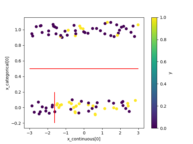
Visualize the stochastic data generative model and generated samples.

Note that values of categorical features will be shown with jitters.

Parameters:

filenamestr, optional: Filename for saving the figure, by default None
formatstr, optional: Rendering output format ("pdf", "png", …).
sample_sizeint, optional: A positive integer, by default 100
x_continuousnumpy.ndarray, optional: A 2-dimensional float array whose size is (sample_size,c_dim_continuous), by default None.
x_categoricalnumpy.ndarray, optional: A 2-dimensional int array whose size is (sample_size,c_dim_categorical), by default None. Each element x_categorical[i,j] must satisfy 0 <= x_categorical[i,j] < self.c_num_children_vec[self.c_dim_continuous+j].

See also

graphviz.Digraph

Examples

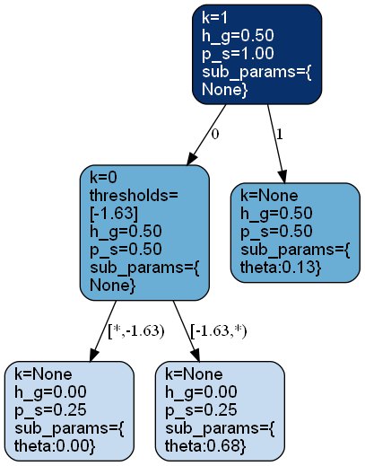
>>> from bayesml import metatree
>>> model = metatree.GenModel(
>>>     c_dim_continuous=1,
>>>     c_dim_categorical=1)
>>> model.gen_params(threshold_type='random')
>>> model.visualize_model()

class bayesml.metatree.LearnModel(c_dim_continuous, c_dim_categorical, c_max_depth=2, c_num_children_vec=2, c_num_assignment_vec=None, c_ranges=None, SubModel=<module 'bayesml.bernoulli'>, sub_constants={}, h0_k_weight_vec=None, h0_g=0.5, sub_h0_params={}, h0_metatree_list=[], h0_metatree_prob_vec=None)#

Bases: Posterior, PredictiveMixin

The posterior distribution and the predictive distribution.

Parameters:

c_dim_continuousint: A non-negative integer
c_dim_categoricalint: A non-negative integer
c_max_depthint, optional: A positive integer, by default 2
c_num_children_vecnumpy.ndarray, optional: A vector of positive integers whose length is c_dim_continuous+c_dim_categorical, by default [2,2,…,2]. The first c_dim_continuous elements represent the numbers of children of continuous features at inner nodes. The other c_dim_categorial elements represent those of categorical features. If a single integer is input, it will be broadcasted.
c_num_assignment_vecnumpy.ndarray, optional: A vector of positive integers whose length is c_dim_continuous+c_dim_categorical. The first c_dim_continuous elements represent the maximum assignment numbers of continuous features on a path. The other c_dim_categorial elements represent those of categorical features. If it has a negative element (e.g., -1), the corresponding feature will be assigned any number of times. By default [-1,…,-1].
c_rangesnumpy.ndarray, optional: A numpy.ndarray whose size is (c_dim_continuous,2). A threshold for the k-th continuous feature will be generated between c_ranges[k,0] and c_ranges[k,1]. By default, [[-3,3],[-3,3],…,[-3,3]].
SubModelclass, optional: bernoulli, categorical, poisson, normal, exponential, or linearregression, by default bernoulli
sub_constantsdict, optional: constants for self.SubModel.LearnModel, by default {}
h0_k_weight_vecnumpy.ndarray, optional: A vector of positive real numbers whose length is c_dim_continuous+c_dim_categorical, by default [1,…,1].
h0_gfloat, optional: A real number in $[0, 1]$, by default 0.5
sub_h0_paramsdict, optional: h0_params for self.SubModel.LearnModel, by default {}
h0_metatree_listlist of metatree._Node, optional: Root nodes of meta-trees, by default []
h0_metatree_prob_vecnumpy.ndarray, optional: A vector of real numbers in $[0, 1]$ that represents prior distribution of h0_metatree_list, by default uniform distribution Sum of its elements must be 1.0.

Attributes:

c_dim_features: int: c_dim_continuous + c_dim_categorical
hn_k_weight_vecnumpy.ndarray: A vector of positive real numbers whose length is c_dim_continuous+c_dim_categorical
hn_gfloat: A real number in $[0, 1]$
sub_hn_paramsdict: hn_params for self.SubModel.LearnModel
hn_metatree_listlist of metatree._Node: Root nodes of meta-trees
hn_metatree_prob_vecnumpy.ndarray: A vector of real numbers in $[0, 1]$ that represents prior distribution of h0_metatree_list. Sum of its elements is 1.0.

Methods

`calc_feature_importances`()	Calculate the feature importances
`calc_pred_density`(y)	Calculate the values of the probability density function of the predictive distribution.
`calc_pred_dist`([x_continuous, x_categorical])	Calculate the parameters of the predictive distribution.
`calc_pred_var`()	Calculate the variance of the predictive distribution.
`estimate_params`([loss, visualize, filename, ...])	Estimate the parameter under the given criterion.
`fit`([x_continuous, x_categorical, y, alg_type])	Fit the model to the data.
`get_constants`()	Get constants of LearnModel.
`get_h0_params`()	Get the hyperparameters of the prior distribution.
`get_hn_params`()	Get the hyperparameters of the posterior distribution.
`get_p_params`()	Get the parameters of the predictive distribution.
`load_h0_params`(filename)	Load the hyperparameters to h0_params.
`load_hn_params`(filename)	Load the hyperparameters to hn_params.
`make_prediction`([loss])	Predict a new data point under the given criterion.
`overwrite_h0_params`()	Overwrite the initial values of the hyperparameters of the posterior distribution by the learned values.
`pred_and_update`([x_continuous, ...])	Predict a new data point and update the posterior sequentially.
`predict`([x_continuous, x_categorical])	Predict the data.
`predict_proba`([x_continuous, x_categorical])	Predict the data.
`reset_hn_params`()	Reset the hyperparameters of the posterior distribution to their initial values.
`save_h0_params`(filename)	Save the hyperparameters using python `pickle` module.
`save_hn_params`(filename)	Save the hyperparameters using python `pickle` module.
`set_h0_params`([h0_k_weight_vec, h0_g, ...])	Set the hyperparameters of the prior distribution.
`set_hn_params`([hn_k_weight_vec, hn_g, ...])	Set the hyperparameters of the posterior distribution.
`update_posterior`([x_continuous, ...])	Update the hyperparameters of the posterior distribution using traning data.
`visualize_posterior`([filename, format, ...])	Visualize the posterior distribution for the parameter.

get_constants()#

Get constants of LearnModel.

Returns:

constantsdict of {str: int, numpy.ndarray}

"c_dim_continuous" : the value of self.c_dim_continuous
"c_dim_categorical" : the value of self.c_dim_categorical
"c_num_children_vec" : the value of self.c_num_children_vec
"c_max_depth" : the value of self.c_max_depth
"c_num_assignment_vec" : the value of self.c_num_assignment_vec
"c_ranges" : the value of self.c_ranges

set_h0_params(h0_k_weight_vec=None, h0_g=None, sub_h0_params=None, h0_metatree_list=None, h0_metatree_prob_vec=None)#

Set the hyperparameters of the prior distribution.

Parameters:

h0_k_weight_vecnumpy.ndarray, optional: A vector of positive real numbers whose length is c_dim_continuous+c_dim_categorical, by default None.
h0_gfloat, optional: A real number in $[0, 1]$, by default None
sub_h0_paramsdict, optional: h0_params for self.SubModel.LearnModel, by default None
h0_metatree_listlist of metatree._Node, optional: Root nodes of meta-trees, by default None
h0_metatree_prob_vecnumpy.ndarray, optional: A vector of real numbers in $[0, 1]$ that represents prior distribution of h0_metatree_list, by default None. Sum of its elements must be 1.0.

get_h0_params()#

Get the hyperparameters of the prior distribution.

Returns:

h0_paramsdict of {str: float, list, dict, numpy.ndarray}

"h0_k_weight_vec" : the value of self.h0_k_weight_vec
"h0_g" : the value of self.h0_g
"sub_h0_params" : the value of self.sub_h0_params
"h0_metatree_list" : the value of self.h0_metatree_list
"h0_metatree_prob_vec" : the value of self.h0_metatree_prob_vec

set_hn_params(hn_k_weight_vec=None, hn_g=None, sub_hn_params=None, hn_metatree_list=None, hn_metatree_prob_vec=None)#

Set the hyperparameters of the posterior distribution.

Parameters:

hn_k_weight_vecnumpy.ndarray, optional: A vector of positive real numbers whose length is c_dim_continuous+c_dim_categorical, by default None.
hn_gfloat, optional: A real number in $[0, 1]$, by default None
sub_hn_paramsdict, optional: hn_params for self.SubModel.LearnModel, by default None
hn_metatree_listlist of metatree._Node, optional: Root nodes of meta-trees, by default None
hn_metatree_prob_vecnumpy.ndarray, optional: A vector of real numbers in $[0, 1]$ that represents prior distribution of hn_metatree_list, by default None. Sum of its elements must be 1.0.

get_hn_params()#

Get the hyperparameters of the posterior distribution.

Returns:

hn_paramsdict of {str: float, list, dict, numpy.ndarray}

"hn_k_weight_vec" : the value of self.hn_k_weight_vec
"hn_g" : the value of self.hn_g
"sub_hn_params" : the value of self.sub_hn_params
"hn_metatree_list" : the value of self.hn_metatree_list
"hn_metatree_prob_vec" : the value of self.hn_metatree_prob_vec

update_posterior(x_continuous=None, x_categorical=None, y=None, alg_type='MTRF', **kwargs)#

Update the hyperparameters of the posterior distribution using traning data.

Parameters:

x_continuousnumpy.ndarray, optional

A 2-dimensional float array whose size is (sample_size,c_dim_continuous), by default None.

x_categoricalnumpy.ndarray, optional

A 2-dimensional int array whose size is (sample_size,c_dim_categorical), by default None. Each element x_categorical[i,j] must satisfy 0 <= x_categorical[i,j] < self.c_num_children_vec[self.c_dim_continuous+j].

ynumpy.ndarray

values of objective variable whose dtype may be int or float

alg_type{‘MTRF’, ‘given_MT’, ‘MTMCMC’, ‘REMTMCMC’}, optional

type of algorithm, by default ‘MTRF’

**kwargsdict, optional

optional parameters of algorithms, by default {}.

When alg_type='MTRF'
- In MTRF[1], sklearn.ensemble.RandomForestClassifier or sklearn.ensemble.RandomForestRegressor is called as a subroutine. Arguments given as **kwargs are passed to these subroutines. Therefore, if you want to specify options for these subroutines, e.g., n_estimators or random_state, etc., you can specify them here. However, max_depth of these subroutines is set to the value of self.c_max_depth, so if you set it again, you will get an error.
When alg_type='given_MT'
- There are no optional parameters for 'given_MT'.
When alg_type='MTMCMC'
- burn_in : int
  
  The length of the burn-in phase, by default 100.
- num_metatrees : int
  
  The number of sampling after burn-in phase, by default 500.
- g_max : float
  
  An initial value of a parameter to controll the entropy of the proposal distribution in the Metropolis-Hastings step, by default 0.0. See also Appendix B.4 in [2]. g_max will be tuned in burn-in phase by Algorithm 1 in [2].
- rho : float
  
  Parameter of Algorithm 1 in [2], by default 0.99.
- phi : float
  
  Parameter of Algorithm 1 in [2], by default 0.999.
- p_obj : float
  
  Parameter of Algorithm 1 in [2], by default 0.3. p_obj corresponds to $r_\mathrm{obj}$ in Algorithm 1 in [2].
- threshold_type : {‘1d_kmeans’, ‘sample_midpoint’}
  
  A generating rule of thresholds for continuous explanatory variables, by default '1d_kmeans'. See also Appendix G in [2].
- seed : {None, int}, optional
  
  A seed to initialize numpy.random.default_rng(), by default None.
When alg_type='REMTMCMC'
- burn_in : int
  
  The length of the burn-in phase, by default 100.
- num_metatrees : int
  
  The number of sampling after burn-in phase, by default 500.
- num_chains : int
  
  Number of replicas in replica exchange Monte Carlo Methods, by default 8. It corresponds to $J$ in Appendix D in[2]
- g_max : float
  
  A parameter to controll the entropy of the proposal distribution in the Metropolis-Hastings step, by default 0.9. In contrast to MTMCMC, g_max tuning is not performed in burn-in phase. See also Appendix B.4 in [2].
- beta_vec : {None, numpy.ndarray}
  
  Temperature parameters for replica exchange Monte Carlo methods, by default None. It must satisfy $0 \leq \beta_1 < \beta_2 < \cdots < \beta_J = 1$. If None, $\beta_j = j/J$. See also Appendix D in [2].
- num_interval : int
  
  Length of interval between replica exchange processes, by default 10. See also Appendix D in [2].
- num_exchange : int
  
  Number of replicas exchanged in a single replica exchange process, by default 4. See also Appendix D in [2].
- threshold_type : {‘1d_kmeans’, ‘sample_midpoint’}
  
  A generating rule of thresholds for continuous explanatory variables, by default '1d_kmeans'. See also Appendix G in [2].
- seed : {None, int}, optional
  
  A seed to initialize numpy.random.default_rng(), by default None.

See also

sklearn.ensemble.RandomForestClassifier
sklearn.ensemble.RandomForestRegressor

References

[1]

Dobashi, N., Saito, S., Nakahara, Y., & Matsushima, T. (2021). Meta-Tree Random Forest: Probabilistic Data-Generative Model and Bayes Optimal Prediction. Entropy, 23(6), 768. Available from https://doi.org/10.3390/e23060768

[2]

Nakahara, Y., Saito, S., Ichijo, N., Kazama, K. & Matsushima, T. (2025). Bayesian Decision Theory on Decision Trees: Uncertainty Evaluation and Interpretability. Proceedings of The 28th International Conference on Artificial Intelligence and Statistics, in Proceedings of Machine Learning Research 258:1045-1053 Available from https://proceedings.mlr.press/v258/nakahara25a.html.

estimate_params(loss='0-1', visualize=True, filename=None, format=None)#

Estimate the parameter under the given criterion.

The approximate MAP meta-tree $M_{T,\boldsymbol{k}_b} = \mathrm{argmax} p(M_{T,\boldsymbol{k}_{b'}} | \boldsymbol{x}^n, y^n)$ will be returned.

Parameters:

lossstr, optional: Loss function underlying the Bayes risk function, by default "0-1". This function supports only "0-1".
visualizebool, optional: If True, the estimated metatree will be visualized, by default True. This visualization requires graphviz.
filenamestr, optional: Filename for saving the figure, by default None
formatstr, optional: Rendering output format ("pdf", "png", …).

Returns:

map_rootmetatree._Node: The root node of the estimated meta-tree that also contains the estimated parameters in each node.

Warning

Multiple metatrees can represent equivalent model classes. This function does not take such duplication into account.

See also

graphviz.Digraph

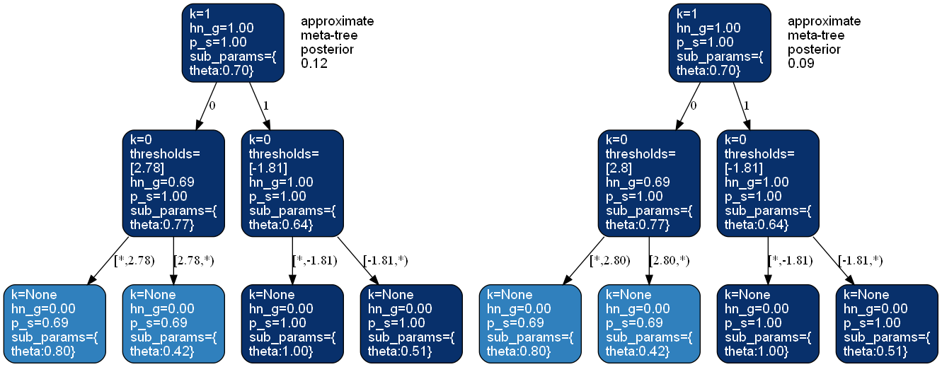
visualize_posterior(filename=None, format=None, num_metatrees=3, h_params=False)#

Visualize the posterior distribution for the parameter.

This method requires graphviz.

Parameters:

filenamestr, optional: Filename for saving the figure, by default None
formatstr, optional: Rendering output format ("pdf", "png", …).
num_metatreesint, optional: Number of metatrees to be visualized, by default 3.
h_paramsbool, optional: If True, hyperparameters at each node will be visualized. if False, estimated parameters at each node will be visulaized.

See also

graphviz.Digraph

Examples

>>> from bayesml import metatree
>>> gen_model = metatree.GenModel(
>>>     c_dim_continuous=1,
>>>     c_dim_categorical=1)
>>> gen_model.gen_params(threshold_type='random')
>>> x_continuous,x_categorical,y = gen_model.gen_sample(200)
>>> learn_model = metatree.LearnModel(
>>>     c_dim_continuous=1,
>>>     c_dim_categorical=1)
>>> learn_model.update_posterior(x_continuous,x_categorical,y)
>>> learn_model.visualize_posterior(num_metatrees=2)

get_p_params()#

Get the parameters of the predictive distribution.

This model does not have a simple parametric expression of the predictive distribution. Therefore, this function returns None.

Returns:

None

calc_pred_dist(x_continuous=None, x_categorical=None)#

Calculate the parameters of the predictive distribution.

Parameters:

x_continuousnumpy.ndarray, optional: A 2-dimensional float array whose size is (sample_size,c_dim_continuous), by default None.
x_categoricalnumpy.ndarray, optional: A 2-dimensional int array whose size is (sample_size,c_dim_categorical), by default None. Each element x_categorical[i,j] must satisfy 0 <= x_categorical[i,j] < self.c_num_children_vec[self.c_dim_continuous+j].

make_prediction(loss=None)#

Predict a new data point under the given criterion.

Parameters:

lossstr, optional: Loss function underlying the Bayes risk function, by default None. This function supports “squared”, “0-1”, and “KL”. If loss is None, “squared” is used when the submodel is a regression model (normal, poisson, exponential, or linear regression), and “0-1” is used when the submodel is a classification model (bernoulli or categorical).

Returns:

predicted_valuesnumpy.ndarray

The predicted values under the given loss function. If the submodel is a classification model (bernoulli or categorical) and the loss function is “KL”, the predictive distribution will be returned as numpy.ndarray that consists of occurence probabilities.

The size of the predicted values or the number of predictive distribution is the same as the sample size of x_continuous and x_categorical when you called calc_pred_dist(x_continuous,x_categorical).

pred_and_update(x_continuous=None, x_categorical=None, y=None, loss=None)#

Predict a new data point and update the posterior sequentially.

Parameters:

x_continuousnumpy.ndarray, optional: A 2-dimensional float array whose size is (sample_size,c_dim_continuous), by default None.
x_categoricalnumpy.ndarray, optional: A 2-dimensional int array whose size is (sample_size,c_dim_categorical), by default None. Each element x_categorical[i,j] must satisfy 0 <= x_categorical[i,j] < self.c_num_children_vec[self.c_dim_continuous+j].
ynumpy.ndarray: values of objective variable whose dtype may be int or float
lossstr, optional: Loss function underlying the Bayes risk function, by default None. This function supports “squared”, “0-1”, and “KL”.

Returns:

predicted_valuesnumpy.ndarray

The size of the predicted values or the number of predictive distribution is the same as the sample size of x_continuous and x_categorical when you called calc_pred_dist(x_continuous,x_categorical).

calc_pred_var()#

Calculate the variance of the predictive distribution.

Returns:

varsnumpy.ndarray: The variances of the predictive distribution. The size of the vars is the same as the sample size of x when you called calc_pred_dist(x).

calc_feature_importances()#

Calculate the feature importances

Returns:

feature_importancesnumpy.ndarray: The feature importances.

calc_pred_density(y)#

Calculate the values of the probability density function of the predictive distribution.

Parameters:

ynumpy.ndarray: y must have a size that is broadcastable to (sample_size,), i.e., the size along the last dimension must be 1 or sample_size. Here, sample_size is the sample size of x when you called calc_pred_dist(x).

Returns:

p_ynumpy.ndarray: The values of the probability density function of the predictive distribution.

fit(x_continuous=None, x_categorical=None, y=None, alg_type='MTRF', **kwargs)#

Fit the model to the data.

This function is a wrapper of the following functions:

>>> self.reset_hn_params()
>>> self.update_posterior(x_continuous,x_categorical,y,alg_type,**kwargs)
>>> return self

Parameters:

x_continuousnumpy.ndarray, optional: A 2-dimensional float array whose size is (sample_size,c_dim_continuous), by default None.
x_categoricalnumpy.ndarray, optional: A 2-dimensional int array whose size is (sample_size,c_dim_categorical), by default None. Each element x_categorical[i,j] must satisfy 0 <= x_categorical[i,j] < self.c_num_children_vec[self.c_dim_continuous+j].
ynumpy.ndarray: values of objective variable whose dtype may be int or float
alg_type{‘MTRF’, ‘given_MT’, ‘MTMCMC’, ‘REMTMCMC’}, optional: type of algorithm, by default ‘MTRF’
**kwargsdict, optional: optional parameters of algorithms, by default {}

Returns:

selfLearnModel: The fitted model.

predict(x_continuous=None, x_categorical=None)#

Predict the data.

This function is a wrapper of the following functions:

>>> self.calc_pred_dist(x_continuous,x_categorical)
>>> return self.make_prediction()

Parameters:

x_continuousnumpy.ndarray, optional: A 2-dimensional float array whose size is (sample_size,c_dim_continuous), by default None.
x_categoricalnumpy.ndarray, optional: A 2-dimensional int array whose size is (sample_size,c_dim_categorical), by default None. Each element x_categorical[i,j] must satisfy 0 <= x_categorical[i,j] < self.c_num_children_vec[self.c_dim_continuous+j].

Returns:

predicted_valuesnumpy.ndarray: If the submodel is a regression model (normal, poisson, exponential, or linear regression), the predicted values under the squared loss function will be returned. If the submodel is a classification model (bernoulli or categorical), the predicted values under the 0-1 loss function will be returend. The size of the predicted values is the same as the sample size of x_continuous and x_categorical.

predict_proba(x_continuous=None, x_categorical=None)#

Predict the data.

This function is supported when the submodel is a classification model (bernoulli or categorical). It is a wrapper of the following functions:

>>> self.calc_pred_dist(x_continuous,x_categorical)
>>> return self.make_prediction(loss="KL")

Parameters:

x_continuousnumpy.ndarray, optional: A 2-dimensional float array whose size is (sample_size,c_dim_continuous), by default None.
x_categoricalnumpy.ndarray, optional: A 2-dimensional int array whose size is (sample_size,c_dim_categorical), by default None. Each element x_categorical[i,j] must satisfy 0 <= x_categorical[i,j] < self.c_num_children_vec[self.c_dim_continuous+j].

Returns:

predicted_distributionsnumpy.ndarray: The predicted distributions under the KL loss function. The number of the predicted distributions is the same as the sample size of x_continuous and x_categorical.

bayesml.metatree package

Contents

bayesml.metatree package#

Module contents#

Stochastic Data Generative Model#

Prior Distribution#

Posterior Distribution#

Approximation by MTRF#

Approximation by MTMCMC#

References#